Neural Networks & Embeddings
Transcript
Made automatically from the video's sound, so it may contain mistakes. Click a line to play from there.
Welcome to this explainer. Look, today we're bypassing all the beginner definitions and we are definitely skipping the biological brain metaphors. Instead, we're diving straight into the rigorous maths and system architectures that actually drive deep learning in production.
So, if you're ready to look under the hood of modern neural networks, you are exactly in the right place. So think about this for a second. Why is it that sparse, one hot vectors and basic gradient descent completely fall apart when we throw them at sequence problems at scale?
It's a fundamental failure of both geometry and computation. And honestly, solving that failure is the very foundation of modern AI. Here's our roadmap for today. First, moving from discrete symbols to continuous geometry.
Second, graphs and reverse mode auto diff. Third, pathological landscapes and stabilization. And fourth, memory arithmetic in production. Right, section one, discrete symbols to continuous geometry, moving from sparse to dense representations.
There's a pretty brutal juxtaposition between blind orthogonal one-hot vectors and the continuous spatial geometry of dense embeddings. With a one-hot vector, every single word is just a massive, mostly empty array. The curse of dimensionality kicks in immediately with that OV explosion.
But worse than that, every token is exactly 90 degrees orthogonal to every other token. That means absolutely zero semantic similarity. They literally have nothing in common mathematically.
But when you project those discrete symbols into a much lower dimensional continuous space, suddenly meaning is encoded geometrically. You can actually measure the relationship between concepts just by calculating the cosine similarity or the dot product of their vectors.
It's a real game changer. To see how this works, models like Word to VEC, learn this continuous vector geometry by analysing the context of surrounding words. By using a skipgram architecture alongside noise contrastive estimation, the model essentially figures out that words hanging out in similar contexts should be pulled closer together geometrically.
It completely transforms a discrete string of text into this rich mathematical landscape where spatial relationships mirror actual syntactic and semantic structure. Now it's not a perfect system by any stretch. Static representations run into some serious geometric roadblocks, like an osotropy.
It's this fascinating yet frustrating pathology where vectors unnaturally clump together into narrow little cones within high dimensional space, which severely limits their expressiveness. Plus a static model assigns the exact same vector to a word, regardless of its context.
As you can imagine, this completely fails on polysemy, where a single word has entirely different meanings depending on how it's actually being used. Graphs and reverse mode autodiff. This is our computational engine.
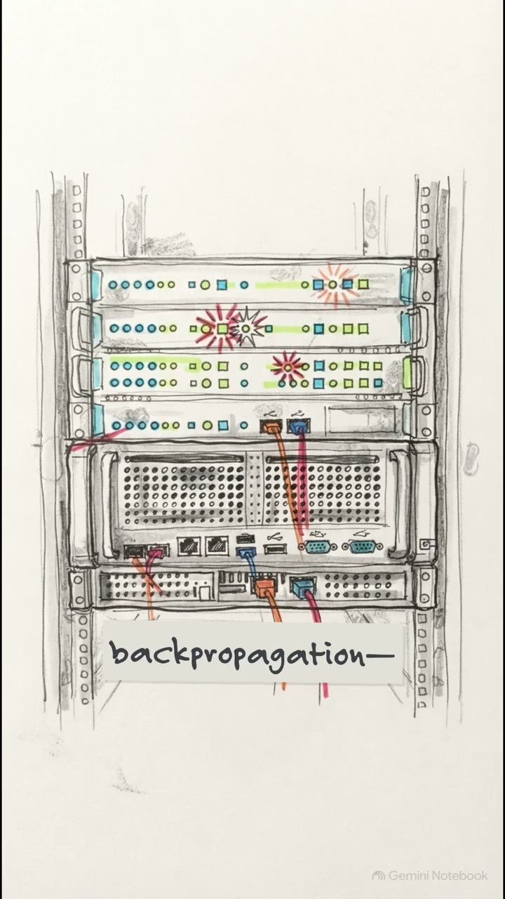
Look, backpropagation, or reverse mode automatic differentiation, is literally the only reason deep learning is computationally tractable. As Christopher Oler brilliantly points out, it can make training with gradient descent as much as 10 million times faster.
Without this highly specific algorithm, training a modern neural network wouldn't just be a bit slow. It would quite literally outlast the lifespan of the engineers building it. 200,000 years versus a week.
That is the scale we are talking about here. Let's break down the computational graph. During the forward pass, you're computing your logits and your cross entropy loss, but you absolutely must cache the intermediate matrix outputs, the activations, directly in VRAM.
Why? Because you are going to need them for the backward pass. This is exactly why training demands so much heavy-duty hardware compared to simple inference.
The backward pass then uses the chain rule and Jacobian vector products to map out exactly how every single weight contributed to that final scalar loss. And this is where the massive efficiency kicks in. Reverse mode autodiff costs a constant O of one passes relative to your parameter count, just to compute gradients for a single scalar loss.
Think about it. If we used forward mode differentiation on a model with a million parameters, we'd have to pass through that graph a million times. Reverse mode lets us update all million weights in one single, elegant backward sweep.
Alright, section three. Pathological landscapes and stabilization. Time to fix the engine. Honestly, the lost landscape of a deep neural network is incredibly hostile.
But the good news is every mathematical pathology has a specific engineered solution. Standard vanilla SGD just zigzags wildly when it hits high curvature, ill-conditioned Hessian ravines.
So how do we fix it? We use exponential moving averages in momentum and adaptive scaling in Atom W. When sequential data causes vanishing or exploding gradients, we introduce the additive cell state gates you see in LSTMs.
The rule is simple. Every time the math breaks down, we engineer a specific architectural bridge to bypass the pathology. If you want to build a truly robust architecture, residual connections and layer norm are just clever little tricks.
They are mandatory physical foundations. By adding the original input back to the output of a layer, you're giving the gradient an identity shortcut, right? It can flow backwards without being completely crushed by repeated nonlinearities and matrix multiplications.
Pair that shortcut with layer normalization to keep the variance strictly bounded, and you've basically paved a highly stable gradient highway through hundreds of layers. Let's move to our final section.
Section 4. Memory arithmetic and production, the real infrastructure costs. Because at the end of the day, all these beautiful mathematical models actually have to run on silicon, and the byte per parameter arithmetic is totally unforgiving.
A full ADOM training pass consumes up to eight times more VRAM than simple inference. In production inference, you basically just need memory for the master weights. But during training, it's a whole different story.
You need space for the weights, the gradients, the ADAM optimizers first and second moments, and as we discussed, massive amounts of memory for those cached forward activations. This brutal arithmetic dictates literally every engineering decision you make.
You're constantly forced to balance embedding dimensions, batch sizes, and model complexity against very strict physical constraints. Want to increase your batch size to reduce gradient noise? Well, your memory footprint just spiked.
Opting for highly contextualized representations over static ones? Your latency increases. It is just a continuous tug of war between the mathematical ideal you want and the actual physical limits of your GPUs.
So I'm going to leave you with this final thought to apply to your own systems. Bigger isn't always better. Where does the decision boundary actually lie for your next deployment? If you're just doing clustering, similarity search, or basic classification, spinning up a massive, memory hungry, generative LLM might be absolute overkill.
A highly tuned, lightweight, dense embedding model will probably do the job faster, cheaper, and with a fraction of the VRAM. Ultimately, deeply understanding the maths beneath the architecture is what empowers you to make that call.