Vector Databases Explained
Transcript
Made automatically from the video's sound, so it may contain mistakes. Click a line to play from there.
Welcome back to The Explainer. Today we're cutting right through all that AI hype to look at the concrete systems engineering realities of modern vector databases. We're bypassing the magic and focusing strictly on the actual mechanics of storing and searching embeddings at scale.
Just to quickly recap our previous explainer, we built change data capture, or CDC event pipelines, which are exactly what feed these derived embedding indexes in production. If your source of truth is Postgres, your CDC pipeline is synchronizing that data straight into these vector structures.
Vector storage and bugs inside ANN, metadata filtering, memory math, and engine comparison, and finally decision boundaries. Let's dive into part one vector storage and production bugs. Now we are going to completely skip the introductory LLM prompt tutorials today.
If you need a refresher on RAG context, go check out AI Basics, Season 1, Episode 4. Instead, we have to ask a fundamental database question. Why is it that a team will stand up a shiny new vector cluster only to immediately suffer from stale permission leaks and zero result queries?
Well, it starts with why standard B trees completely fall apart when we hit 768 or 1536 dimensional space. The answer is the curse of dimensionality. In high-dimensional Euclidean space, the distance between any two points starts to look roughly the same, which makes traditional tree-based spatial divisions utterly useless.
Right, part two. Inside ANN index structures. Let's open up the hood and look at the computational mechanics. The core trade-off here is moving away from exact KNN.
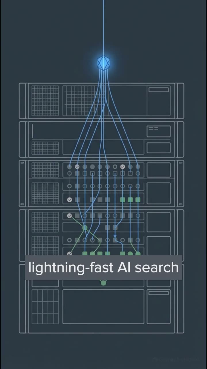
Exact KNN is a brutally slow SIMD flat scan, where the compute complexity is O of N vectors times D dimensions. Instead, we move to approximate nearest neighbour, or ANN techniques. With ANN, we sacrifice a tiny controlled sliver of recall to achieve lightning fast millisecond query latency.
We essentially stop looking for the absolute mathematically closest point and settle for good enough. One major approach to this is IVF, or inverted file index. It works in two steps.
First, it clusters your vectors into K-means volonoi cells, which are defined by centroids called NList. At search time, it only looks inside the closest buckets. But here is the catch.
If your true nearest neighbour happens to be just across the boundary in an adjacent cell, you'll miss it entirely. To fix this, you crank up the n probe parameter, forcing the system to search multiple nearby clusters.
You're trading a bit of speed for much higher recall. This brilliantly illustrates the academic benchmark curves of IVF ADC versus FLAN from the NeurIPS papers. It maps out the exact trade-off between search time on the vertical axis and search quality, or recall, on the horizontal.
By tuning the shortlist size and the number of core centroids, you allow these algorithms to operate at radically different latency and accuracy trade-offs, completely crushing older FLAN methods. Now, this is where it gets really interesting.
Comparing the industry standard, HNSW, against disk ANN. It reveals a massive architectural divide. HNSW builds a multi layer navigable small world graph. It's incredibly fast and accurate, governed by connection limits and candidate pool sizes, but it is heavily RAM dependent.
Disk ANN, on the other hand, relies on a Vamina graph structure, designed specifically to live on NVMe SSDs, keeping only highly compressed product quantization codes in memory. It completely bypasses RAM limits, meaning you can search a billion points on a single workstation.
A real game changer. Metadata filtering and quantization. So what happens when you try to filter these dense graphs using a standard where clause, like a specific tenant ID?
Well, the crucial point is that naive filtering literally breaks vector search. If you pre-filter, meaning you remove nodes from the graph before searching, you destroy the HNSW graph connectivity. The path to your destination is severed.
But if you post-filter, finding the nearest neighbors first and then discarding mismatches, you're often going to return fewer than K matches or even zero matches if your wear clause is too strict. To fix this system-breaking reality, dedicated engines like QDrant and Weavate use what's called filterable HNSW.
They extend the graph with additional edges based on indexed payload values, often using boring bitmaps, which lets you traverse the graph whilst applying filters. Alternatively, PG vector 0.8 and above handles this via iterative index scans. It basically just keeps automatically scanning more of the index until your strict limit is actually met.
Let's get into part four. Worked memory and cost math. We need to drop the it scales well marketing fluff for a second and look at the brutal quantified memory math.
Because in systems engineering, memory is money. If you have 25 million 1,536-dimensional vectors from a standard embedding model, and you're storing them in 32-bit floats with a 35% HNSW graph overhead, that is going to demand roughly 207 gigabytes of pinned RAM.
That is a massive, incredibly expensive memory footprint for just 25 million rows. But look how the memory footprint just melts away for 10 million vectors when we move down the quantization ladder. We drop from 83GB in 32-bit floats down to roughly 42GB using half EC, all the way down to just 21 gigabytes if we use scalar intake quantization.
You can even take it down to one-bit binary quantization with oversampled rescoring, squeezing it into just a few gigabytes. This kind of compression is absolutely vital for running at scale. The vector engine comparison.
Armed with that math, let's stack these architectural options directly against each other. Dedicated engines like QDrant, Milvis, Weave, and Pinecone are absolutely brilliant at handling 50 million to a billion plus vectors.
They offer purpose-built sharding and advanced disk ANN capabilities, but they come with the operational tax of dual store CDC sync lag. Conversely, running PG vector inside Postgres gives you zero CDC lag, strict acid transactional joins for permissions, and shared backups.
The trade-off? It hits a ceiling when your HNSW build memory starts competing with your primary database operations. Finally, part six, decision boundaries.
Let's talk about when you absolutely do not need a dedicated vector database. Engineers love to overengineer, don't we? So let's establish some rigid boundaries. If you have under 100k vectors per tenant, do not build a complex ANN graph.
Just use exact flat scans. Modern CPUs with SIMD instructions can chew through that in literal milliseconds. And if your primary requirement is strict acid metadata joins and you have under roughly 5 million to 50 million vectors, staying inside your existing Postgres instance using PG Vector absolutely beats the operational nightmare of syncing a second distributed cluster.
Furthermore, if you are doing exact SKU lookups, part numbers, or highly specific industry jargon queries, pure dense cosine similarity will completely fail you. It's terrible at exact keyword matching. You absolutely must rely on a hybrid search that pairs lexical BM25 with dense vectors, combining those scores using reciprocal rank fusion, or RRF.
Sometimes all you really need is standard Postgres full text search. So evaluate your true scale, your quantization strategy, and your filtering needs first. Before we tee up our next explainer on running data stores in production, I want you to look at your architecture and ask yourself a final brutally honest question.
Are you needlessly paying the operational sync tax of a dedicated vector cluster when your existing infrastructure is actually more than enough? Food for thought. See you in the next one.